scRNAseq normalization

Introduction

scRNA sequencing is a relatively novel technique added to the Biologist's toolkit that allows one to quantitatively probe the "Statistical Mechanics" of Biology. In contrast to traditional bulk RNAseq techniques, which provide population averages, scRNAseq technology measures the complete ensemble of cellular gene expression. Consequently, considerable activity has been focused on mapping the taxonomy of cell states; projects such as the Human Cell Atlas promise to provide a complete enumeration of microscopic cell types within the human body. However, despite recent progress, scRNAseq data have many numerous technical limitations and sources of statistical bias that must be considered before any downstream analysis. The sources of noise within the data include, but are not limited to:

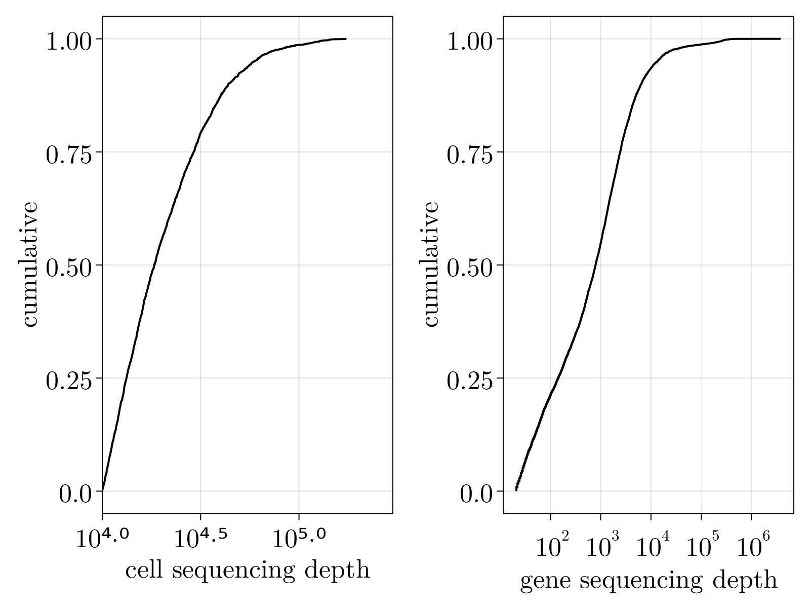
Sequence depth bias: PCR and reverse transcription efficiency will vary across reactions, resulting in artificial variation of sequencing depth across different cells.
Amplification bias: PCR primers are not perfectly random. As a result, some genes will amplify preferentially over others. This will distort the underlying expression distribution.
Batch effect: scRNAseq runs have non-trivial distortions causing cells within a given sequencing run to have greater correlation within than across batches.
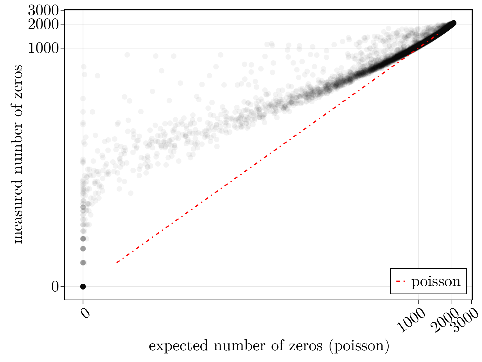
Dropout: Due to molecular competition in the underlying amplification reactions, some genes will fail to amplify during PCR due to early losses. This will lead to more zeros in the resulting count matrix than you would expect by chance.

These biases are approximately rectified by a preprocessing step known as normalization. At a coarse level, all such methods can be thought of as transforming the obtained count matrix from absolute numbers into an estimate of differential expression, i.e. a comparison of a count relative to the measured distribution. Such a procedure is analogous to that of the z-score of a univariate normally-distributed random variable; however, in the case of scRNAseq data, we don't have access to the underlying sampling distributions a priori, it must be estimated empirically. The choice of sampling prior, and details of how the distribution is estimated, delineate normalization practices.

Overview of current methods

TODO: FILL OUT

Our approach

We model the count matrix $n_{\alpha,i}$, where $\alpha$ and $i$ indexes cells and genes respectively, obtained from scRNA sequencing as an unknown, low-rank mean $\mu_{\alpha,i}$ with additive full-rank noise $\delta_{\alpha,i}$ that captures all unknown technical noise and bias.

\[ \tag{1} n_{\alpha,i} = \mu_{\alpha,i} + \delta_{\alpha,i} \]

Our goal during the normalization procedure is two-fold:

Estimate the low-rank mean $\mu_{\alpha,i}$.
Estimate the sampling variance $\langle\delta_{\alpha,i}^2\rangle$ of the experimental noise. Brackets denote an average over (theoretical) realizations of sequencing. This will eventually require an explicit model.

Given both quantities, normalization over gene and cell-specific biases can be achieved by imposing the variances of all marginal distributions to be one. Specifically, we rescale all counts by cell-specific $c_\alpha$ and gene-specific $g_i$ factors $\tilde{n}_{\alpha,i} \equiv c_\alpha n_{\alpha,i} g_i$ such that

\[ \tag{2} \displaystyle\sum\limits_{\alpha} \langle \tilde{\delta}_{\alpha,i}^2 \rangle = \displaystyle\sum\limits_{\alpha}c_\alpha^2 \langle \delta_{\alpha,i}^2 \rangle g_i^2 = N_g \quad \text{and} \quad \displaystyle\sum\limits_{i} \langle \tilde{\delta}_{\alpha,i}^2 \rangle = \displaystyle\sum\limits_{i}c_\alpha^2 \langle \delta_{\alpha,i}^2 \rangle g_i^2 = N_c\]

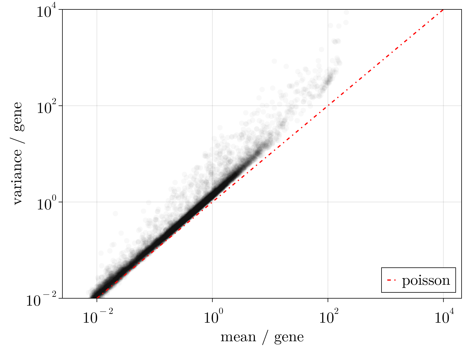
This system of equations can be solved by the Sinkhorn-Knopp algorithm, provided we have a model for $\langle\delta_{\alpha,i}^2\rangle$ parameterized by measurables. Within this formalism, this choice of model fully determines the normalization scheme. Owing to dropout and other sources of overdispersion, as shown empircally in the figure below, we model scRNAseq counts as sampled from an empirically estimated Heteroskedastic Negative Binomial distribution.

Case studies

Before detailing our explicit algorithm, it is helpful to consider a few simpler examples. In the following sections, homoskedastic is used to denote count matrices whose elements are independent and identically distributed (iid), while heteroskedastic denotes more complicated scenarios where each element has a unique distribution.

Homoskedastic Gaussian

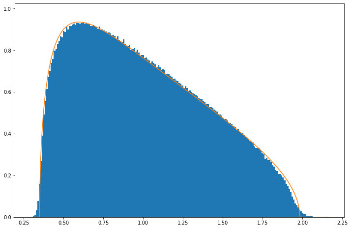
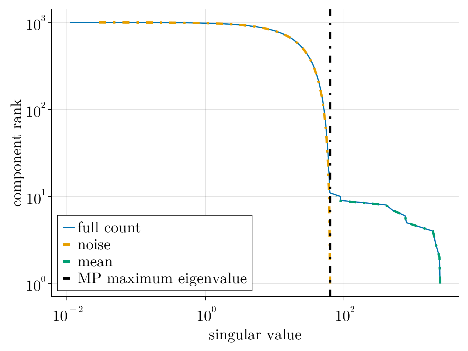
This is slight perturbation of canonical random matrix theory and will serve as a useful pedagogical starting point. Assume $\mu_{\alpha,i}$ is a quenched, low-rank matrix and each element of $\delta_{\alpha,i}$ is sampled from a Gaussian with zero mean and variance $\sigma^2$. In this limit, Eq.(1) reduces to the well-studied spiked population covariance model.

If $\mu_{\alpha,i} = 0$, the spectral decomposition of the count matrix $n_{\alpha,i}$ would be given by the Marchenko-Pastur distribution asymptotically. As such, singular values would be bounded by $\bar{\lambda} \equiv 1+\sigma\sqrt{N_g/N_c}$.

Marchenko pastur distribution (orange) vs random matrix eigenvalues (blue)

Now consider the case of a rank 1 mean, i.e. 1 cell type in the data.

\[ n_{\alpha,i} = \gamma x_\alpha \bar{x}_i + \delta_{\alpha,i}\]

It has been shown^[1]^[2] that this model exhibits the following asymptotic phase transition:

If $\gamma \le \bar{\lambda}$, the top singular value of $n_{\alpha,i}$ converges to $\bar{\lambda}$. Additionally, the overlap of the left and right eigenvector with $x$ and $\bar{x}$ respectively converge to 0.
If $\gamma > \bar{\lambda}$, the top singular value of $n_{\alpha,i}$ converges to $\gamma + \bar{\lambda}/\gamma$. Additionally, the overlap of the left and right eigenvector with $x$ and $\bar{x}$ respectively converge to $1-(\bar{\lambda}/\gamma)^2$

This procedure can generalized to higher rank spike-ins; sub-leading principal components can be found by simply subtracting the previously inferred component from the count matrix $n_{\alpha,i}$. As such, we can only expect to meaningful measure the principal components of $\mu_{\alpha,i}$ that fall above the sampling noise floor, given by the Marchenko-Pastur distribution. Consequently, this forces us to define the statistically significant rank of the count matrix. This is exhibited empirically below.

Heteroskedastic Poisson

The above results have been shown to hold for non-Gaussian Wigner noise matrices^[3], provided each element is still iid. This is manifestly not the case we care about; the normalization procedure must account for heterogeneous sampling variances across both cells and genes. However, it has been shown^[4]^[5] that the distribution of eigenvalues converges almost surely to the Marchenko-Pastur distribution, provided the constraint of Eq.(2) is satisfied! In other words, the eigenvalues of a heteroskedastic matrix is expected converge to that of a random Wigner matrix, provided the row and column variances are uniform (set to unity for convenience).

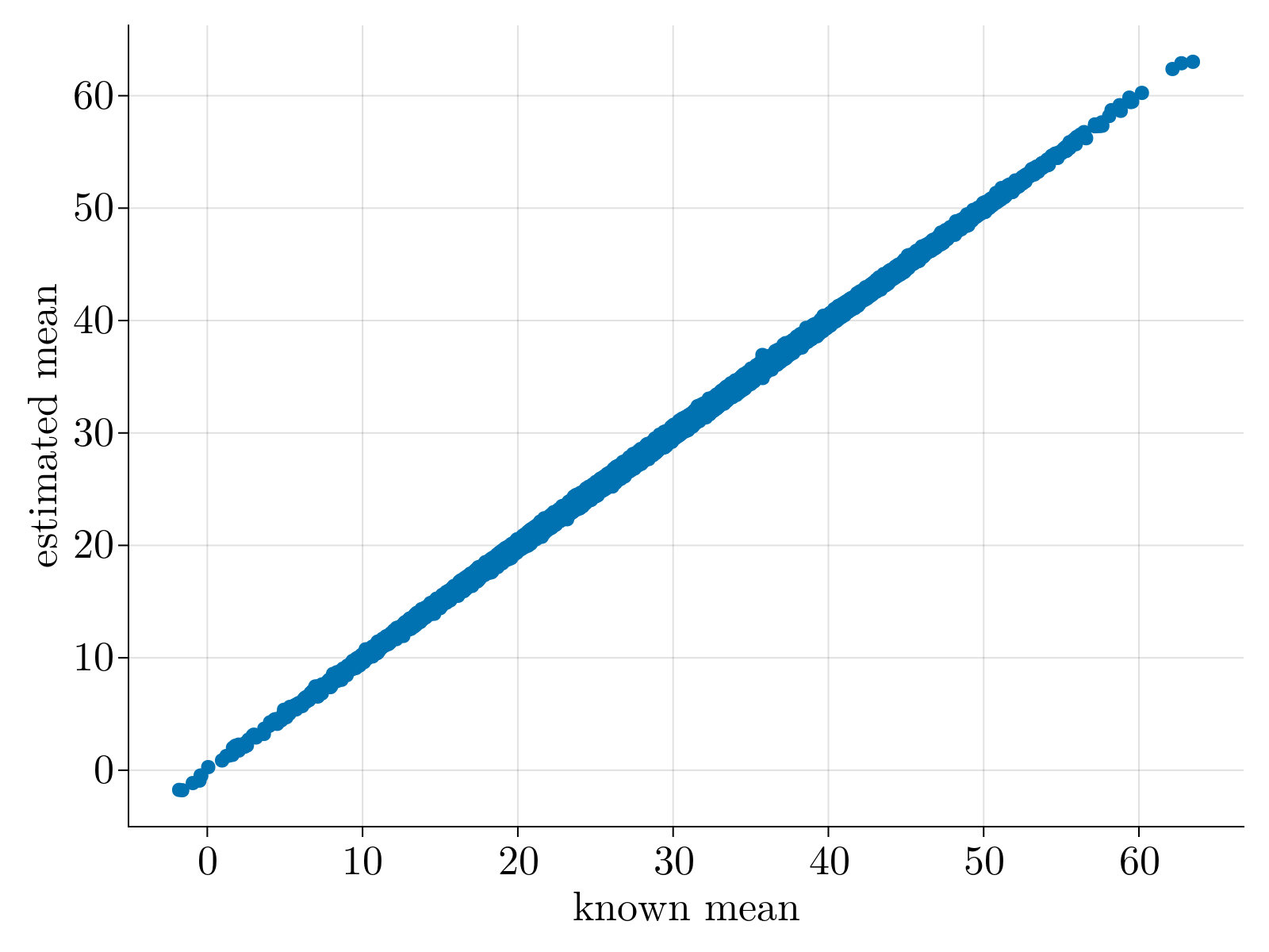
For the remainder of this section, assume the count matrix is sampled from a Poisson distribution, such that $\langle\delta_{\alpha,i}^2\rangle = \mu_{\alpha,i}$. As $n_{\alpha,i}$ is an unbiased estimator for the mean $\mu_{\alpha,i}$, Eq (2) reduces to

\[\displaystyle\sum\limits_{\alpha}c_\alpha^2 n_{\alpha, i} g_i^2 = N_g \quad \text{and} \quad \displaystyle\sum\limits_{i}c_\alpha^2 n_{\alpha,i} g_i^2 = N_c\]

which provides an explicit system of equations to estimate the scaling factors $c_\alpha$ and $g_i$. Once obtained, $\tilde{\mu}_{\alpha,i}$ can be estimated via singular value decomposition of $c_\alpha n_{\alpha,i} g_i$; all components with singular value greater than $\bar{\lambda} = \sqrt{N_c}+\sqrt{N_g}$ can be confidently attributed to the "true mean" $\mu_{\alpha,i}$ while all other components fall amongst the noise. An example is shown below:

Heteroskedastic Negative Binomial

A negative binomial distribution is often used to model overdispersed count data, i.e. a process in which the variance grows superlinearly with the mean. Canonically the distribution arises from the distribution of the number of successes (with probabiliy $p$) obtained after $\Theta_3$ failures of a Bernoulli process. However, the generative stochastic process can equivalently be modelled as an underlying Poisson process in which the emission rate is itself a stochastic variable drawn from a Gamma distribution. This allows us to analytically continue $\Theta_{3}$ from an integer to the reals. Provided we have estimated the mean $\mu_{i\alpha}$ and the overdisperson factor $\Theta_{3;i}$, the unbiased estimator for the variance is given by

\[ \tag{3} \langle \delta_{i\alpha}^2 \rangle = \mu_{i\alpha}\left(\frac{1 + \mu_{i\alpha}\Theta_{3;i}}{1 + \Theta_{3;i}}\right)\]

Direct substitution into Eq. (2) would provide the necessary cell-specific $c_\alpha$ and gene-specific $g_i$ scaling factors.

Empirical sampling distribution

In order to normalize the estimated sampling variance, we must formulate a method to fit a negative binomial to the measured count data per gene. We parameterize the distribution as follows:

\[ p\left(n|\mu,\Theta_{3}\right) = \frac{\Gamma\left(n+\Theta_{3}\right)}{\Gamma\left(n+1\right)\Gamma\left(\Theta_{3}\right)}\left(\frac{\mu}{\mu+\Theta_{3}}\right)^n\left(\frac{\Theta_{3}}{\mu+\Theta_{3}}\right)^{\Theta_{3}}\]

All results, unless explicitly stated otherwise, are obtained empirically from scRNAseq data obtained during early Drosophila melongaster embryogenesis.

Generalized linear model

A central complication in modeling the counts of a given gene across cells with the above generative model is that there are confounding variables that require consideration. For the present discussion, we explictly model the hetereogeneous sequencing depth across cells: naively we expect that if we sequenced a given cell with $2\times$ depth, each gene should scale accordingly. As such, we formulate a generalized linear model

\[ \tag{4} \log \mu_{i\alpha} = \Theta_{1;i} + \Theta_{2;i} \log \chi_{\alpha}\]

where $\chi_\alpha$ denotes the total sequencing depth of cell $\alpha$ We note this formulation can be easily extended to account for other confounds such as batch effect or cell type. The likelihood function for cell $\alpha$, gene $i$ is

\[ p\left(n_{i\alpha}|\Theta_{1;i},\Theta_{2;i}, \Theta_{3;i},\chi_\alpha\right) = \frac{\Gamma\left(n_{i\alpha}+\Theta_{3;i}\right)}{\Gamma\left(n_{i\alpha}+1\right)\Gamma\left(\Theta_{3;i}\right)}\left(\frac{\mu_{i\alpha}}{\mu_{i\alpha}+\Theta_{3;i}}\right)^{n_{i\alpha}}\left(\frac{\Theta_{3;i}}{\mu_{i\alpha}+\Theta_{3;i}}\right)^{\Theta_{3;i}}\]

Maximum Likelihood Estimation

$\{\Theta_{1;i}, \Theta_{2;i}, \Theta_{3;i} \}$ represent $3N_g$ parameters we must infer from the data. We note that a priori this problem is overdetermined; our count matrix is sized $N_g \times N_c$ and thus we attempt to estimate all parameters within a maximum likelihood framework. This is equivalent to minimizing (for each gene independently)

\[\begin{aligned} \tag{5} \mathcal{L}_i = \displaystyle\sum\limits_{\alpha} \left(n_{i\alpha} + \Theta_{3;i}\right)\log\left(e^{\Theta_{1;i}}\chi_\alpha^{\Theta_{2;i}} + \Theta_{3;i}\right) - \Theta_{3;i}\log\left(\Theta_{3;i}\right) \\ - n_{i\alpha}\left(\Theta_{1;i} + \Theta_{2;i}\log \chi_\alpha\right) - \log\left(\frac{\Gamma\left(n_{i\alpha}+\Theta_{3;i}\right)}{\Gamma\left(n_{i\alpha}+1\right)\Gamma\left(\Theta_{3;i}\right)}\right) \end{aligned}\]

Empirically it was determined that to provide a robust estimate of all three parameters that our confounding variables $\chi_{\alpha}$ are given by

\[ \chi_\alpha \equiv \exp\left(\langle \log\left(n_{i\alpha}+1\right) \rangle\right) - 1\]

where angle brackets denote the empirical average over genes for cell $\alpha$. Once the parameters $\{\Theta_{1;i}, \Theta_{2;i}, \Theta_{3;i} \}$ are estimated, Eqns. (2-4) can be utilized to estimate the normalized mean count matrix $\tilde{\mu}_{i\alpha}$. This will also immediately teach us the statistically significant rank of the counting matrix.

Synthetic data verification

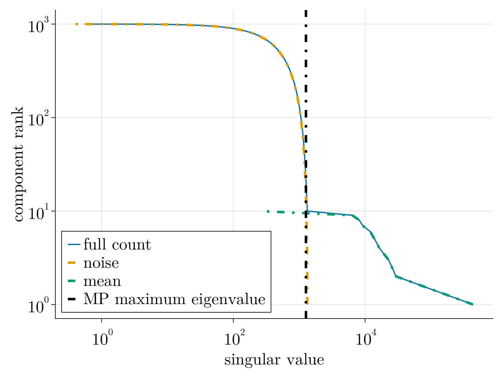
As a first check on the methodology, we generated toy counting data sampled from negative binomial distribution with low rank mean. After estimation of parameters by minimizing Eq. (5), we solved Eq. (2) utilizing our unbiased estimator given by Eq. (3). The result is shown below.

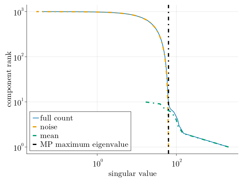
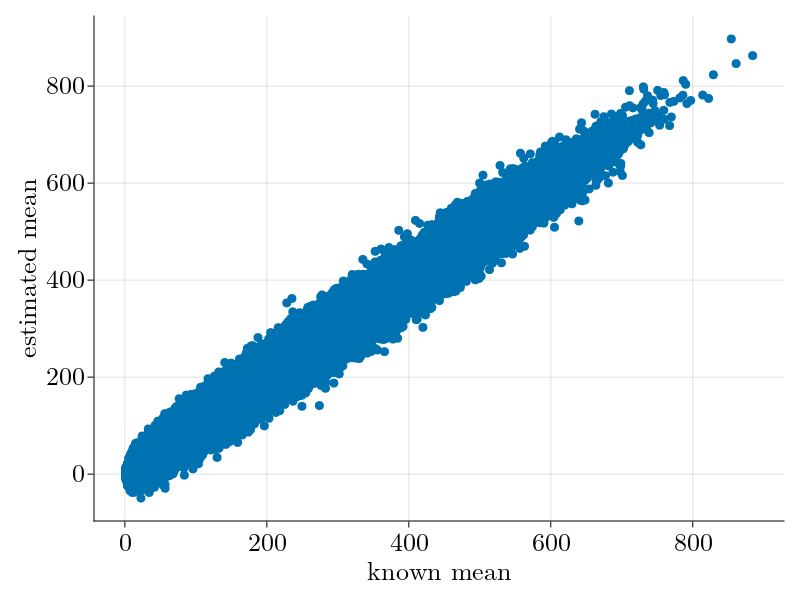
As shown, we underestimate the true rank as a few components have singular values below the Marchenko-Pastur noise floor. This, along with our noisy estimation of the overdispersion factor $\Theta_3$ contributes to our noisier mean estimation when compared to the Poisson case above.

Filter uncertain genes

The uncertainty of our parameter estimates can be computed by the second derivative of the likelihood around our determined minima

\[ \delta \Theta_{a}^2 = \left[\partial_{\Theta_{b}}\partial_{\Theta_{c}} \mathcal{L}\right]^{-1}_{aa}\]

Unsurprisingly, the uncertainty of our estimates for parameters $\{\Theta_{1;i}, \Theta_{2;i}, \Theta_{3;i} \}$ is strongly dependent upon the underlying gene expression; our estimates for lowly expressed genes are highly uncertain. This can be seen in the below figure, which shows the scatter plot of the parameter estimate $\Theta_{a}$ versus its uncertainty $\delta \Theta_a$, colored by the average gene expression.

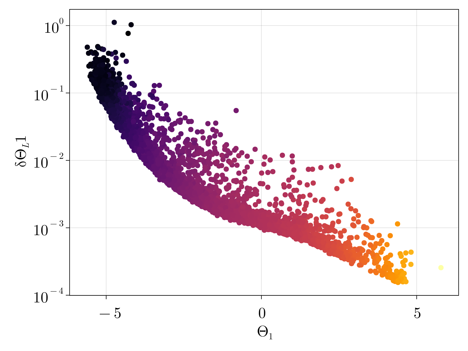
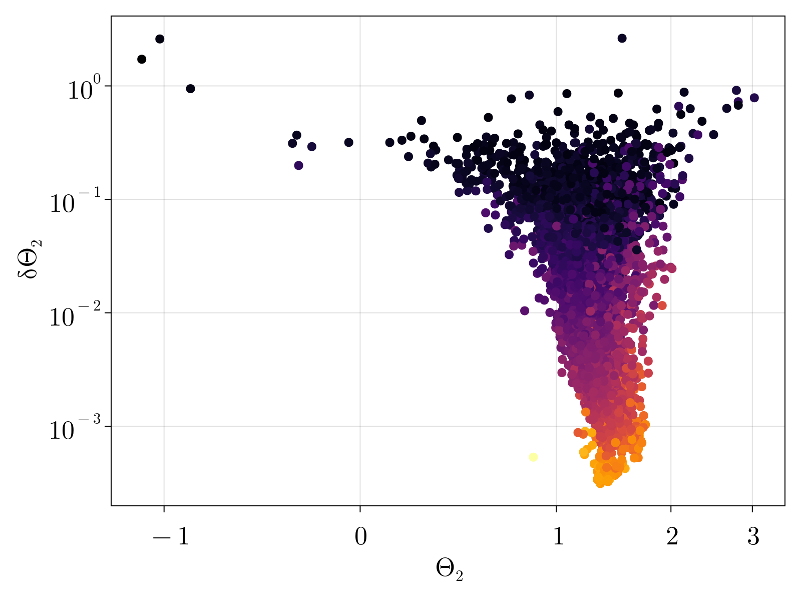
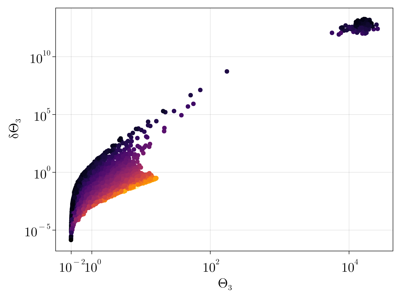
We note that the estimated $\Theta_1$ monotonically grows with increasing gene expression, as was expected by construction. Conversely, the average estimate for $\Theta_2$ shows no obvious trend against expression levels, however the uncertainty $\delta\Theta_2$ monotonically increases with decreasing gene expression. The estimated $\Theta_3$ also appears to be independent of average expression counts with a family of curves with increasing uncertainty defined by decreasing gene levels.

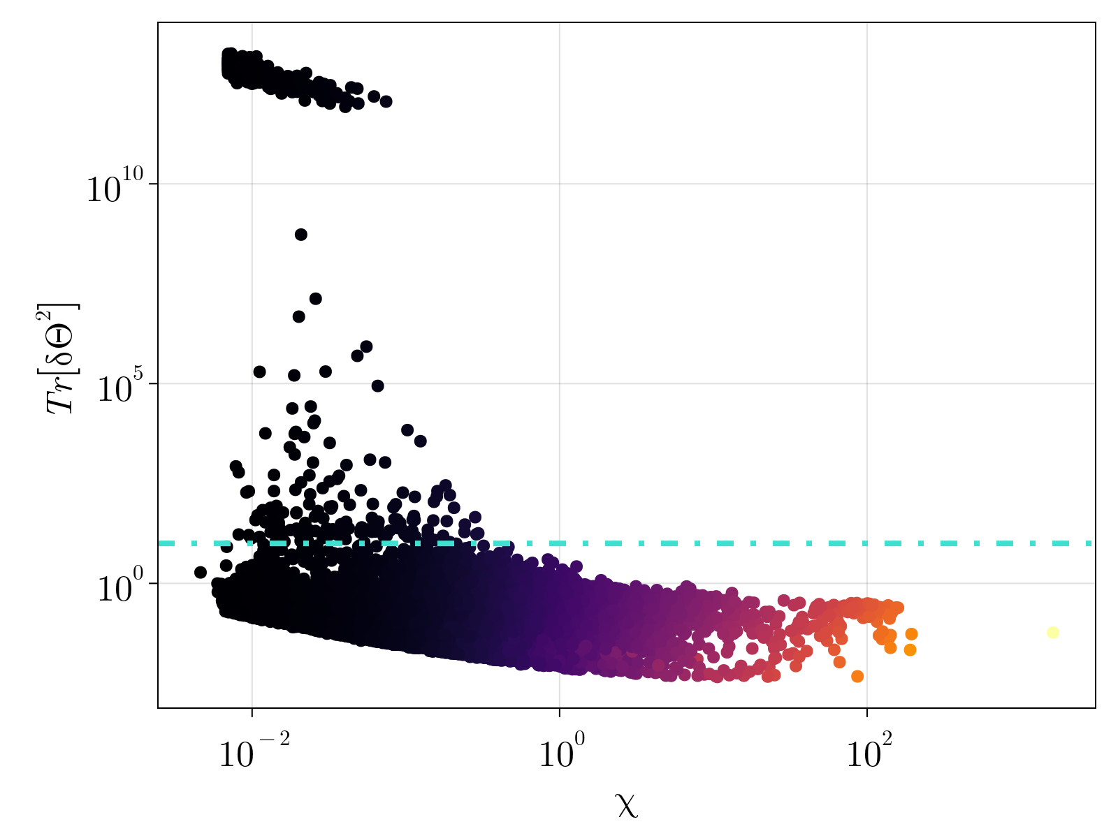
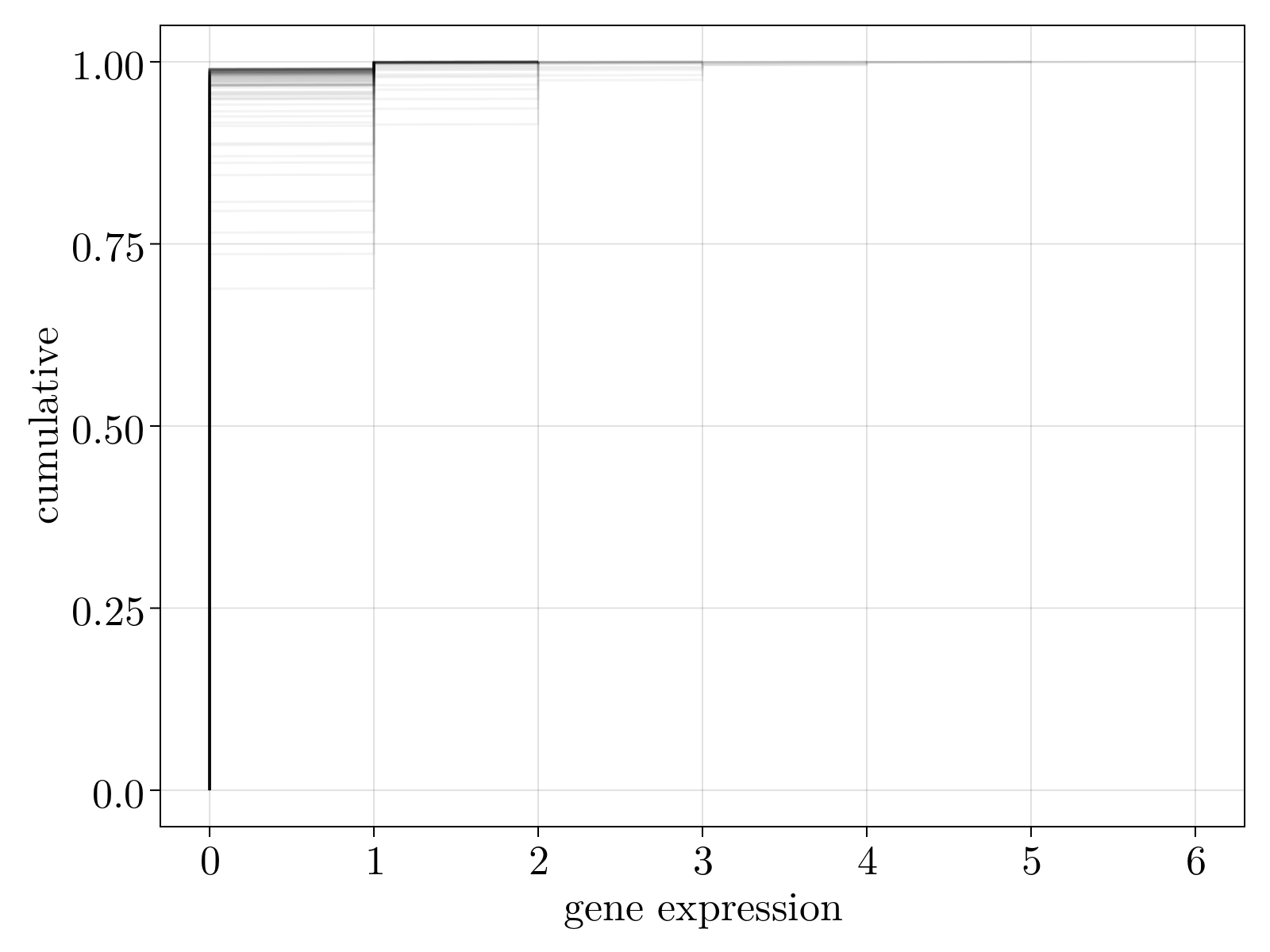
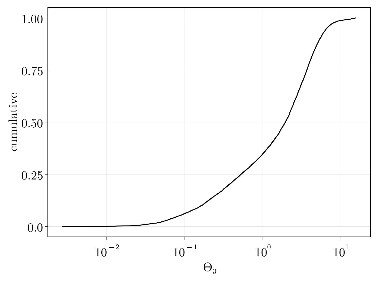
We capture the total uncertainty in our estimates by analyzing the trace of uncertainty $\delta \Theta^2 = \delta \Theta_1^2 + \delta \Theta_2^2 + \delta \Theta_3^2$ A scatter plot of the uncertainty versus average expression level is shown below. We see that expression level is an imperfect predictor of MLE uncertainty. The dashed cyan line denotes our chosen uncertainty cutoff used to remove genes from our count matrix. The right figure displays the cumulative density function for the filtered genes; as can be seen these are lowly expressed genes that are, in practice, 2 state variables.

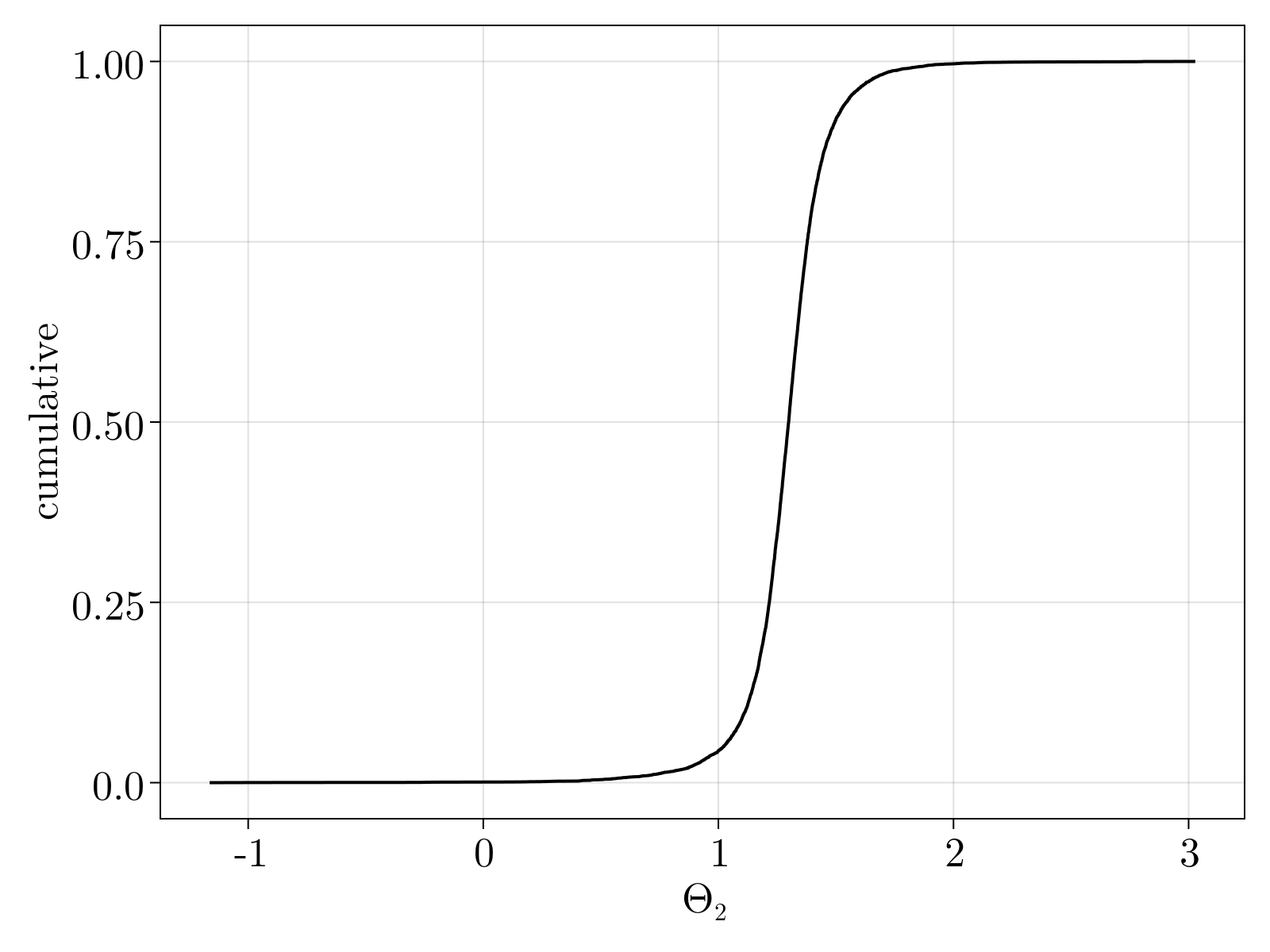
Interestingly, as shown below, the mean estimated value for $\Theta_2$ is slightly higher than 1. This phenomenon persists across all gene expression levels.

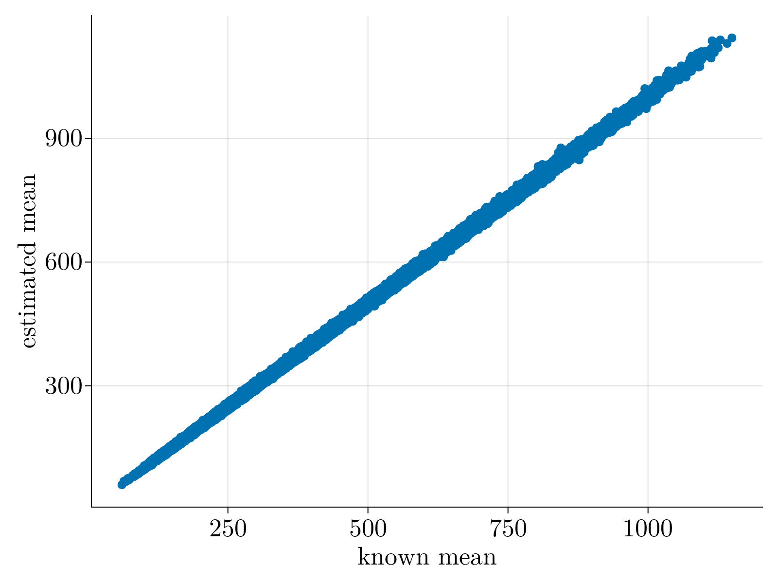
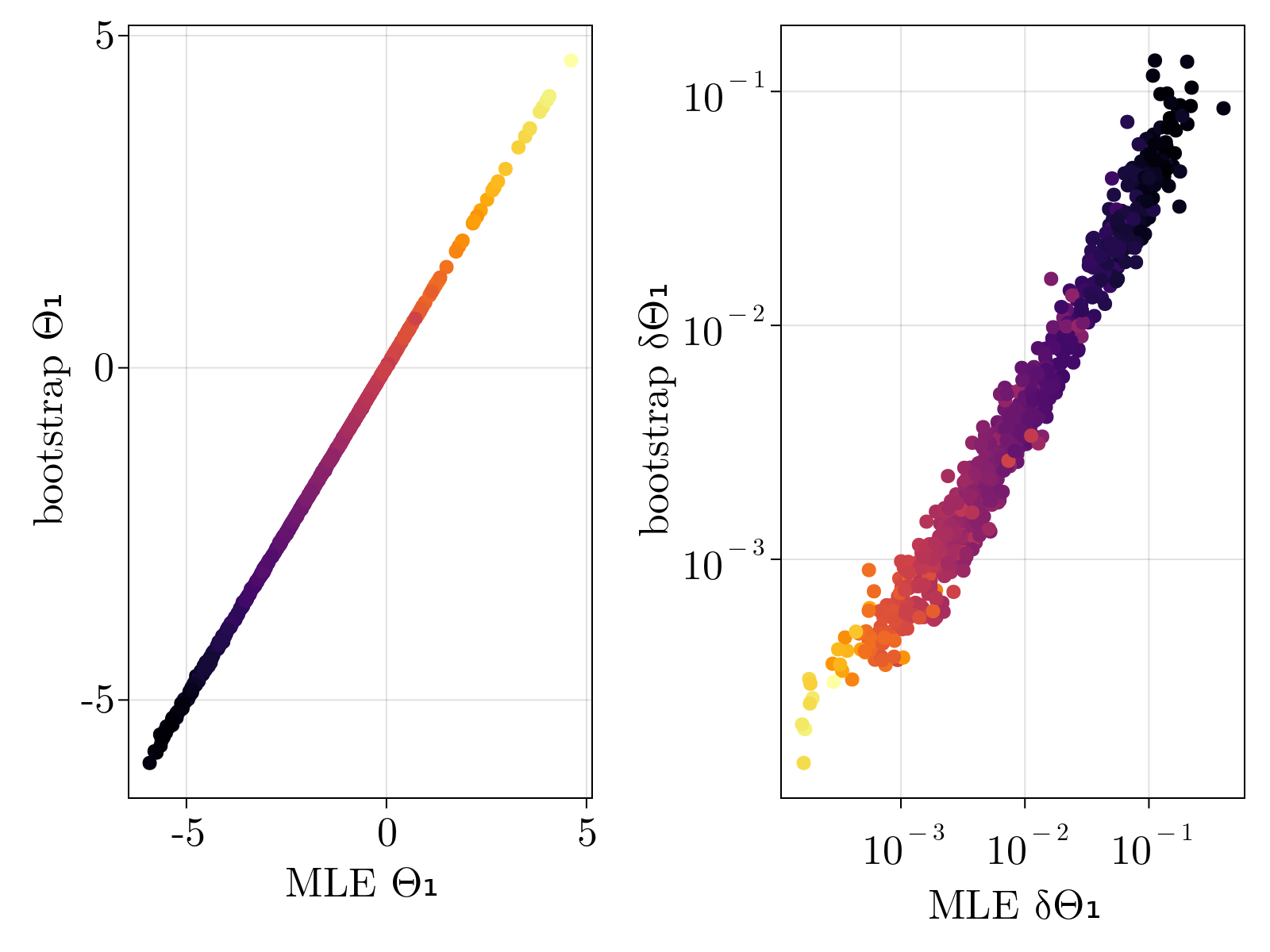
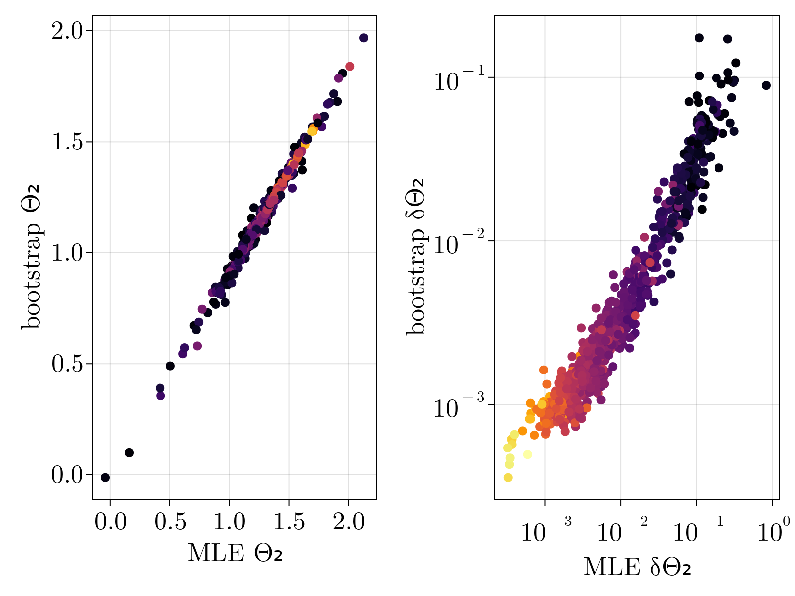
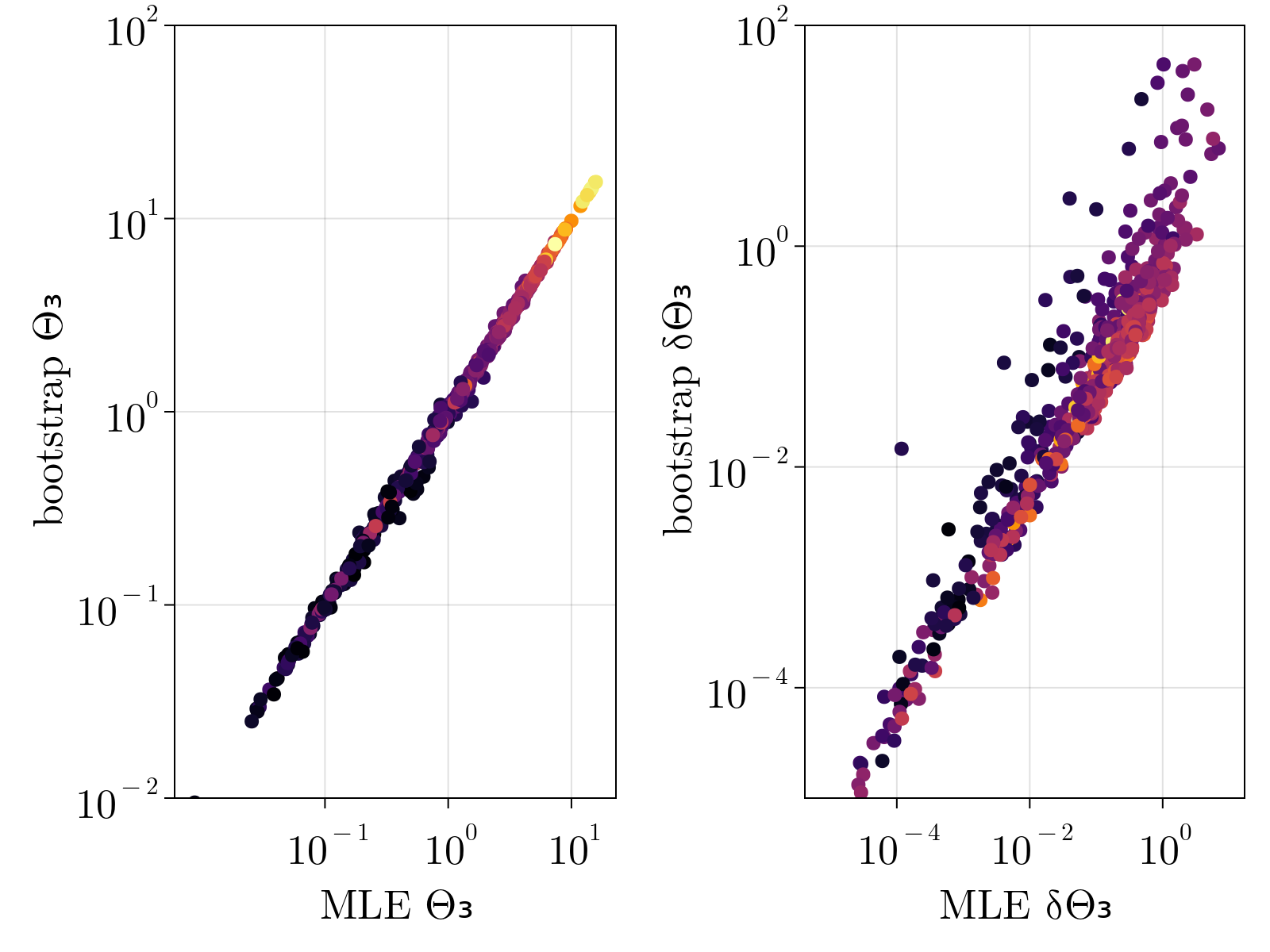
Verify estimates via bootstrap

In order to test that the method does not overfit the data, especially lowly expressed genes, we validated our estimates via bootstrap. Specifically, we re-ran our maximum likelihood estimation of $\{\Theta_{1;i}, \Theta_{2;i}, \Theta_{3;i} \}$ over subsamples of our given set of cells 100 times for each gene. The mean and standard deviation of the resultant empirical distribution was compared directly to our estimates and uncertainty calculations performed on the full dataset. As shown below, we find great quantitative agreement between the empirical estimates and our original calculations, suggesting strongly that we are not overfitting the data.

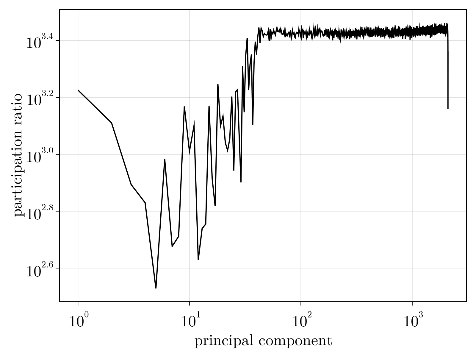
Drosophila results

Just as we performed using the toy data, once parameters $\{\Theta_{1;i}, \Theta_{2;i}, \Theta_{3;i} \}$ are estimated, we can utilize Eqs. (2-5) to normalize the variance matrix and subsequently estimate the mean $\mu_{i\alpha}$. As shown below, we find there are $\sim 30$ statistically significant linear dimensions in the scRNAseq data obtained during early Drosophila melongaster embryogenesis. Interestingly, while not fully delocalized as seen by the participation ratio of the "noise" components, we see that roughly $\sim 1000$ genes contribute significantly to each component suggesting these are coarse "pathways" discovered.

To ensure element-wise positivity, the estimated $\tilde{\mu}_{i\alpha}$ is obtained by performing non-negative matrix factorization on the rescaled $\tilde{n}_{i\alpha}$ with rank $35$. The factorization was initialized using the nndsvda algorithm ^[6] and minimized the least squares objective via a multiplicative update ^[7].

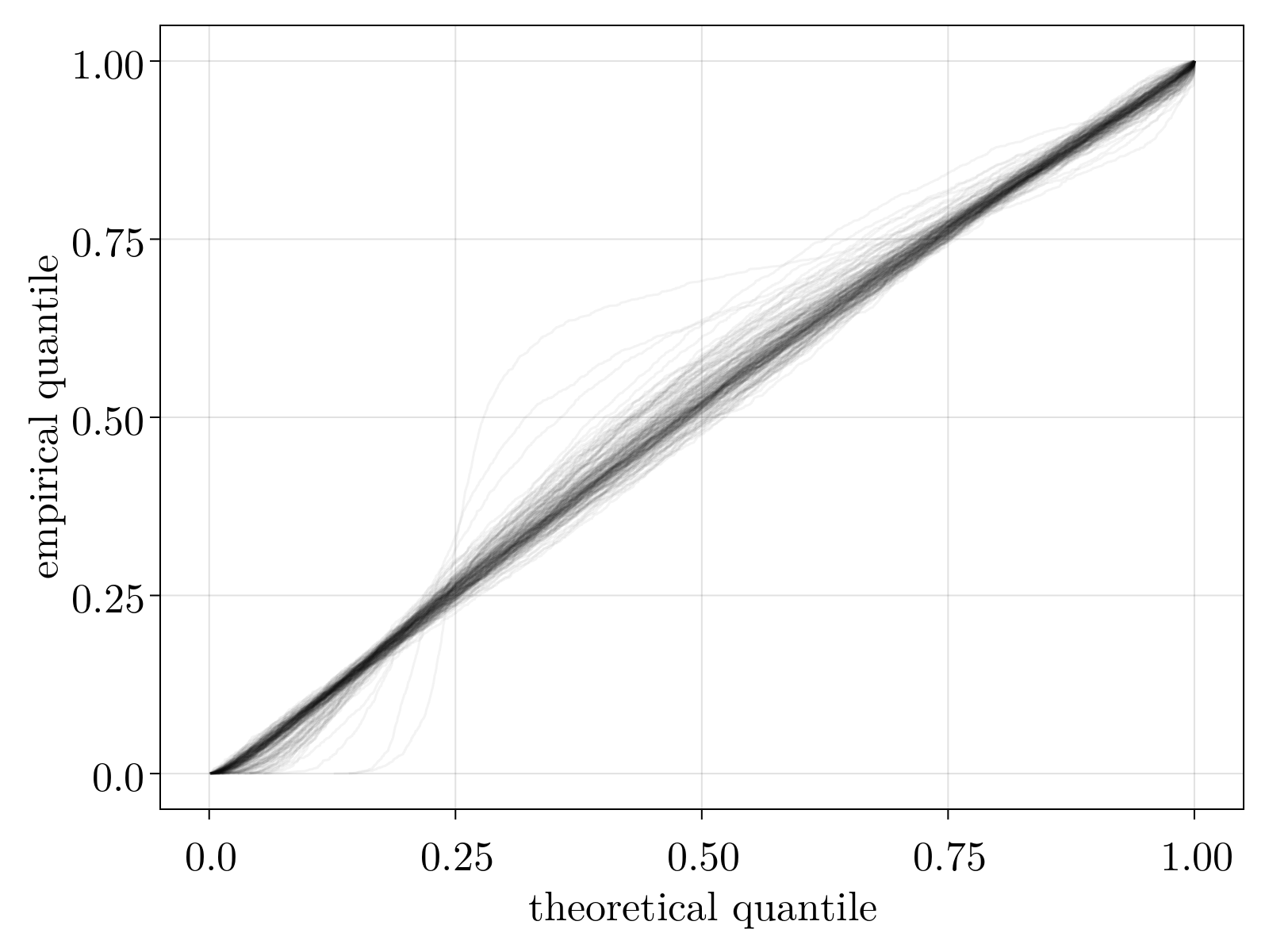
Pearson residuals

Once obtained, $\tilde{\mu}_{i\alpha}$ provides us an estimate for the rescaled mean of the expression of gene $i$ for cell $\alpha$. It is important to note, this will still have gene-specific and cell-specific scales by construction. However, our goal was originally to convert our raw count matrix into more natural units where variation across sequencing depth and gene expression are normalized out. As such, our normalization pipeline requires one last step: convert each rescaled mean into a z-score that measures expression differentially to the observed distribution across cells. Recall that a negative binomial stochastic model is equivalent to a Poisson-Gamma mixture, i.e. a poisson process whose mean is drawn from a Gamma distribution. To this end, we estimate the significance of each $\tilde{\mu}_{i\alpha}$ by fitting a Gamma distribution across cells for each gene, in exactly the same way as we performed for the raw count data with a negative binomial distribution. Specifically, we take the mean to be given by Eq. (4) and minimize the analog of Eq. (5); we omit details here in the interest of brevity. This was determined to be an excellent stochastic model for the computed $\tilde{mu}_{i\alpha}$, as shown by the linear quantile-quantile plot below.

Taken together, our normalized gene count $z_{i\alpha}$ is given by (the mean and variance is given by the estimated Gamma distribution)

\[ \tag{6} z_{i\alpha} \equiv \frac{\tilde{\mu}_{i\alpha} - \mu_{i\alpha}}{\sigma_{i\alpha}}\]