Manifold learning

Introduction

In section scRNAseq spatial inference, we demonstrated that scRNAseq expression data can be directly mapped to space using a reference database of gene expression patterns, provided by the Berkeley Drosophila Transcriptional Network Project. These results motivate a more ambitious question: is positional information directly encoded within gene expression and, as such, can we utilize just scRNAseq counts to infer cellular spatial position de-novo?

We anchor our inference approach on the continuum ansatz of cellular states in a developing embryo. Specifically, we postulate that gene expression is a smoothly varying, continuous function of space, and potentially other continuous degrees of freedom such as time. Said another way, neighboring cells are assumed to be infinitesimally "close" in expression. This formulation is a departure from the conventional, discrete, view of cellular fates taken, for example, in the description of the striped gene patterning observed during the Anterior-Posterior segmentation of the Drosophila melongaster embryo. From our viewpoint, a "discontinuity" of gene expression in a handful of components can also be explained by the curvature of a smooth surface embedded in very high dimensions.

As formulated, spatial inference from scRNAseq data is equivalent to non-linear dimensional reduction: we want to find a small number of degrees of freedom that parameterize the variation across $\sim 10^4$ genes. From Drosophila results, we know that at least minimally, we can describe gene expression within early Drosophila embryogenesis by $31$ relevant components. In this section, we analyze the data within this subspace to show that the data is ultimately generated by an even smaller set of degrees of freedom. Furthermore, we outline a protocol to "learn" this parameterization and show that it can recapitulate space.

Empirical analysis

Hausdorff dimension estimation

A critical parameter to determine empirically is the underlying dimensionality of gene expression of early _Drosophila embryogenesis, as given by the scRNAseq data. Informally, we expect that if the data is sampled from an underlying $d$ dimensional manifold, than the number of points $n$ enclosed by a sphere of radius $R$ should grow as

\[ n(R) \sim R^d\]

However, we note that performing this comparison utilizing the Euclidean metric between normalized cellular expression would be manifestly incorrect; we postulated that gene expression is a manifold which implies a Euclidean metric locally between neighbors. There is no a priori reason to expect Euclidean distances to be a good measure for far cells. Similar considerations hold for other postulated global metrics. Instead, we estimate geodesic distances empirically, in analog to the Isomap algorithm ^[1].

Neighborhood graph construction

The first task is to formulate an algorithm to approximate the metric space the point cloud is sampled from and subsequently utilize our estimate to compute all pairwise distances. We proceed guided by intuition gleaned from Differential Geometry: pairwise distances within local neighborhoods are expected to be well-described by a Euclidean metric in the tangent space. Conversely, macroscopic distances can only be computed via integration against the underlying metric along the corresponding geodesic. We denote $D_{\alpha\beta}$ as the resultant pairwise distances between cell $\alpha,\beta$.

The basic construction of the neighborhood graph is demonstrated in the below cartoon.

Our algorithm to construct the neighborhood graph proceeds in three main steps. First, we visit the local neighborhood of each point (cell) within our dataset. In principle, the neighborhood can be defined by either a fixed number of neighbors $k$ or a given radius $R$. In practice, for Drosophila melongaster we chose to define neighborhood by $k=8$. The neighborhood is assumed to be a good approximation to the manifold tangent space and thus pairwise distances between the point and its neighbors are computed within the euclidean metric. Each pairwise neighborhood relationship is captured by an edge, weighted by the pairwise distance. The collection of all cells, and their neighborhood edges, constitute the neighborhood graph.

Given a neighborhood graph as defined above, computing the "geodesic" distance between cells reduces to finding the shortest path between all pairs of points. This can be solved using either the Floyd-Warshall algorithm in $\mathcal{O}(N^3)$ time ^[2] or iteratively using Dijikstra's algorithm in $\mathcal{O}(N(N\log N + E))$ time ^[3]. We chose the later due to the sparsity of the neighborhood graph. The estimation of geodesic distances, if performed as described, asymptotically approaches the true value as the density of points increases ^[4].

Given our estimate for all pairwise geodesic distances, we can now empirically estimate the Hausdorff dimension. Simply stated, the estimate is done by analyzing the scaling relationship between number of points enclosed within a geodesic ball of radius $R$ and the radius $R$ itself. Below we show the results plotted for each cell within our dataset, along with a trend line $n(R) \sim R^3$ shown in red.

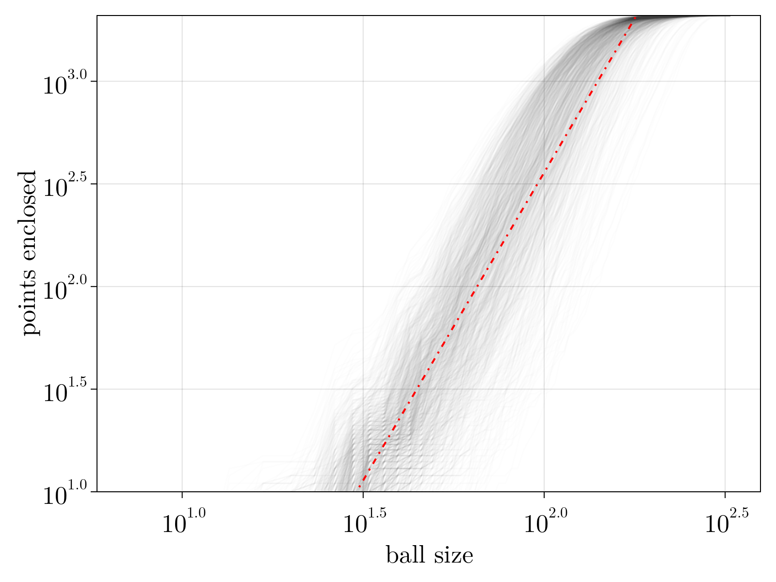
The manifold clearly looks three-dimensional.

Physical proximity implies expression proximity

In Neighborhood graph construction, we demonstrated that the normalized scRNAseq appears to be three-dimensional. This supports half of our continuum ansatz: gene expression of early Drosophila embryogenesis is consistent with being distributed along a low-dimensional manifold. However, a priori is is unclear that such dimensions meaningfully correspond to space. Additionally, at the developmental stage sampled, the Drosophila embryo is a two-dimensional epithelial monolayer and as such it is unclear what a potential third dimension would parameterize. To this end, we utilize the positional labels calculated in scRNAseq spatial inference to assay if physically close cells are close along the putative manifold.

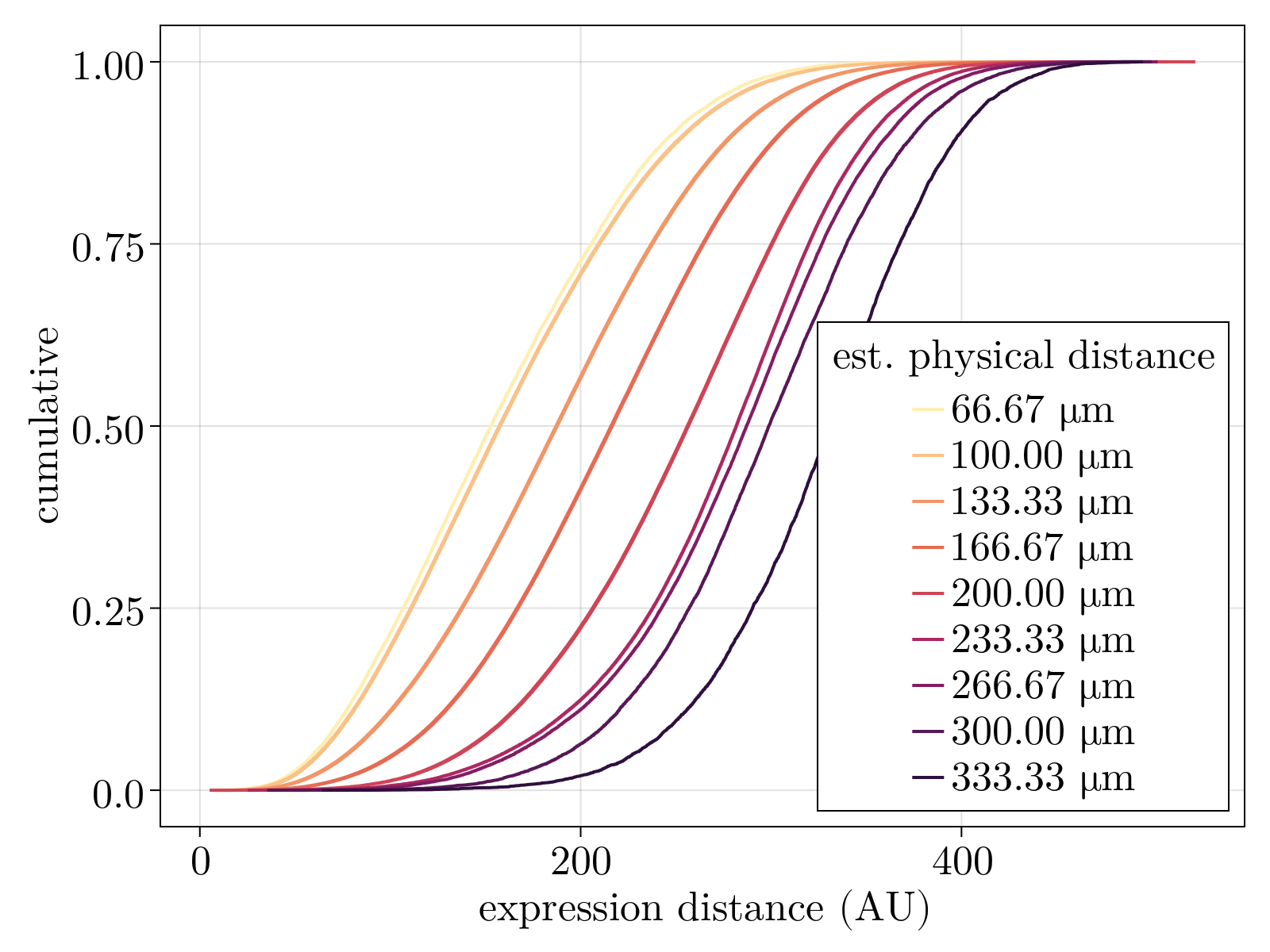
Specifically, we demonstrate that conditioning on varying average spatial geodesic distances results in quantitative effects in the distribution of pairwise expression geodesic distances. Physically close cells are not only close in expression, but the median of the distribution increases quantitatively (albeit non-linearly) with increasing conditioned shells of distance. Taken together, the scRNAseq data is empirically consistent with our continuum expression ansatz.

Isomap dimensional reduction

We provide additional evidence in support of our underlying hypothesis by utilizing the Isomap algorithm ^[1]. As such, we simply perform a Principal Coordinates Analysis on the geodesic distances estimated in Neighborhood graph construction. This is tantamount to finding a set of low-dimensional coordinates $\xi_\alpha$ that minimize the strain between their Euclidean embedding and the given distance matrix $D_{\alpha\beta}$.

\[ E(\{\xi_\alpha\}) = \left(\frac{\left(\sum_{\alpha,\beta} D_{\alpha\beta} - |\xi_\alpha - \xi_\beta|^2\right)^2}{\sum_{\alpha,\beta} D_{\alpha\beta}^2 }\right)^{1/2}\]

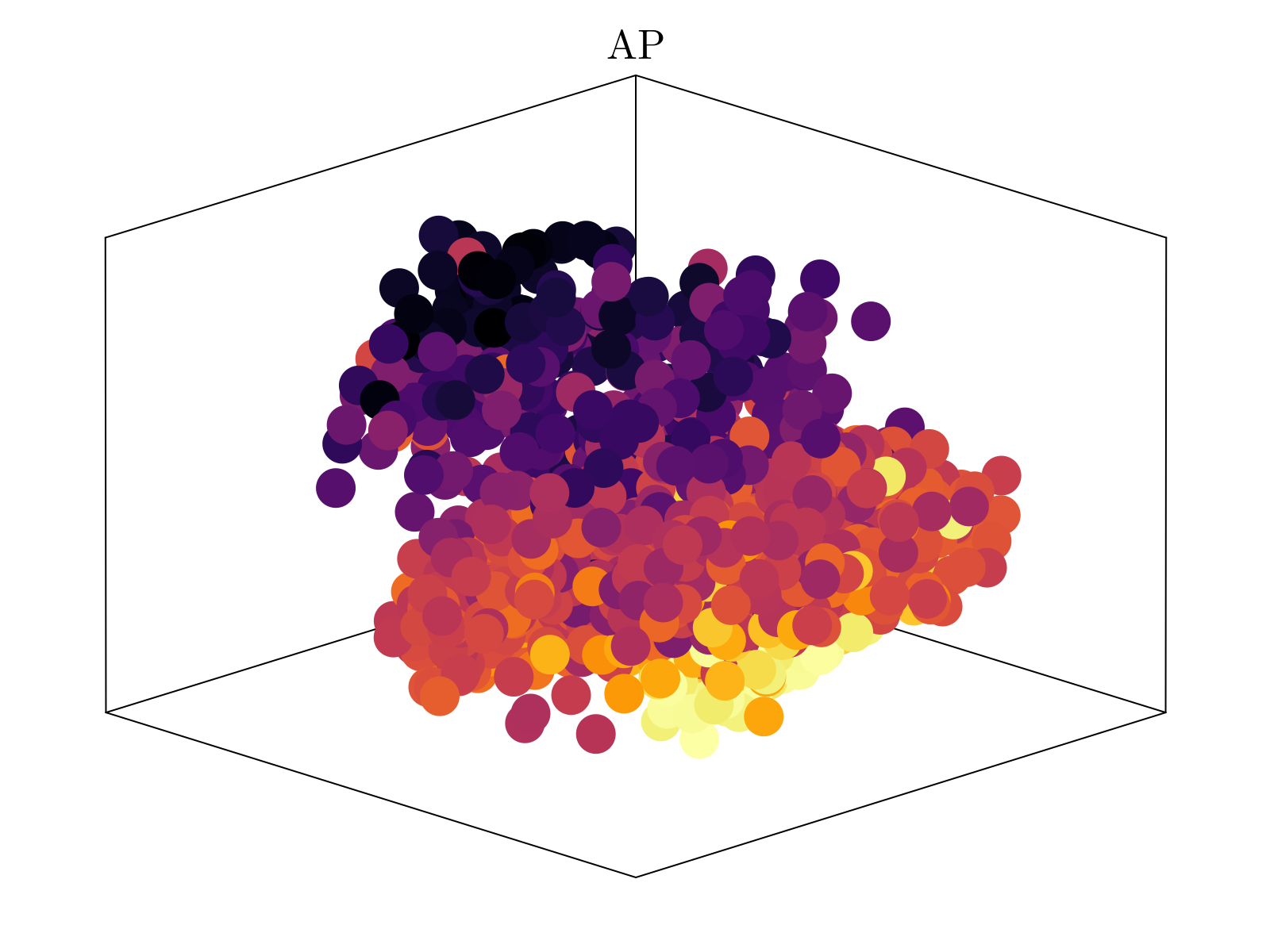
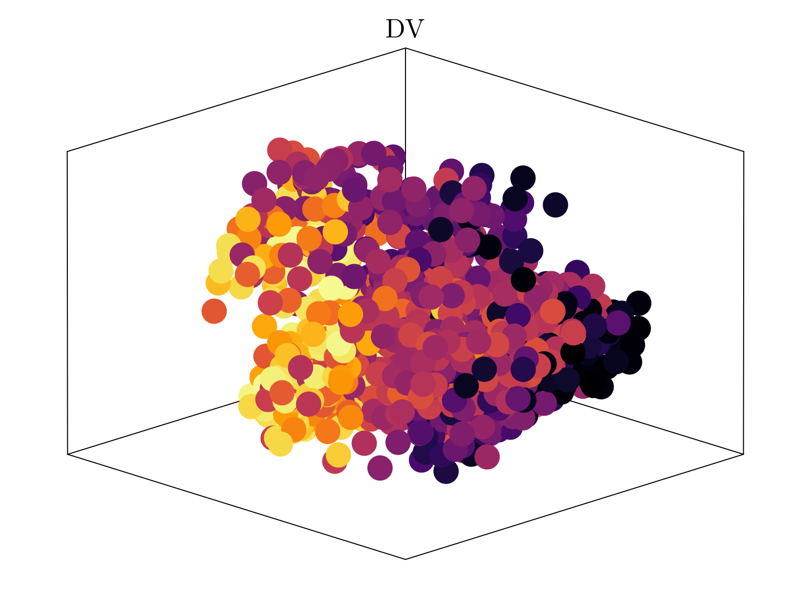
Above, we show the resultant embedding, colored by the estimated AP (anterior-posterior) and DV (dorsal-vental) position, obtained by averaging over the distribution obtained in scRNAseq spatial inference. It is clear that two of the major axes of the embedding quantitatively segregate both spatial axes of the embryo. We emphasize that the estimated spatial positions were not used to generate the shown embedding, but rather only the underlying neighborhood distances of cells within our scRNAseq dataset. This is taken as strong evidence in support of our underlying hypothesis.

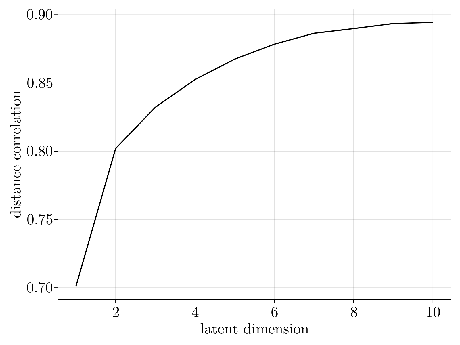
By varying the dimensionality of the Isomap embedding, we see that three dimensions is the "knee" of dimensioning returns, consistent with the 3-dimensional scaling observed above.

De-novo manifold learning

All considerations taken together, we wish to formulate an unsupervised method for nonlinear, dimensional reduction. The natural choice for network architecture is thus an autoencoder ^[5], shown graphically below.

However, in order to enforce the continuum expression ansatz, the neural network should also explicitly conserve the topology of our neighborhood graph; neighborhood rankings should be preserved under the identified mapping. Lastly, we constrain the learned latent representation to be uniformally sampled. This can be viewed as an additional assumption on top of our continuum expression ansatz. Specifically, we assume cells were sampled from the embryonic positions uniformally, i.e. without bias, and, as such, restrict our view to uniformally sampled parameterizations of the underlying expression manifold.

Network architecture

The input to the neural network was the 35 statistically significant components determined in Drosophila results. The encoder layer was designed to be 100 neurons wide and 6 levels deep with dense connections between each layer. In order to prevent overfitting and accelerate training of deep layers, batch normalization was utilized between each latent layer ^[6]. Linear and exponential linear unit activation functions were chosen for the input/output and latent layers respectively. The decoder layer was taken to be mirror symmetric with respect to the encoding layer for simplicity. Training occurred on $80\%$ of the data, batched into groups of $128$ cells. Validation of the resultant network was performed on the remaining $20\%$ to ensure parameters were not overfit. We note that the final results presented here were determined to not be highly sensitive to the specific architectural details outlined here.

Topological conservation

In order to learn an interpretable latent space representation of the intrinsic gene expression manifold, we wish to constrain the estimated pullback to conserve the topology of the input scRNAseq data. This immediately poses the question: what topological features do we wish to preserve from the data to latent space and how do we empirically measure them? The answers immediately determine the additional terms one must add to the objective function used for training.

We opt to utilize an explicitly geometric formalism that will implicitly constrain topology. The intuition for this choice is guided by Differential Geometry: a metric tensor uniquely defines a distance function between any two points on a manifold; the topology induced by this distance function will always coincide with the original topology of the manifold. Thus, by imposing preservation of pairwise distances in the latent space relative to the data, we implicitly conserve topology. It is important to note that this assumes our original scRNAseq data is sampled from a metric space that we have access to. We note that there have been recent promising attempts at designing loss functions parameterized by explicit topological invariants formulated by Topological Data Analysis, e.g. persistent homology. Lastly, one could envision having each network layer operate on a simplicial complex, rather than a flat vector of real numbers, however it is unclear how to parameterize the feed-forward function.

Isometric formulation

The most straightforward manner to preserve distances between the input data and the latent representation is to impose isometry, i.e. distances in both spaces quantitatively agree. This would be achieved by supplementing the objective function with an Isomap analog

\[E_{iso} \sim \displaystyle\sum\limits_{\alpha,\beta} \left(D_{\alpha\beta} - \left|\left| \xi_\alpha - \xi_\beta \right|\right| \right)^2\]

Utilizing this term is problematic for several reasons:

1. Large distances dominate the energetics and as such large-scale features of the intrinsic manifold will be preferentially fit.
2. Generically, $d$ dimensional manifolds can not be isometrically embedded into $\mathbb{R}^d$, e.g. the sphere into the plane. This is seen empirically by the empirical three dimensional scaling but long tail of dimensions seen in the isomap correlation.
3. It trusts the computed distances quantitatively. We simply want close cells to be close in the resultant latent space.

Monometric formulation

Consider a vector $\psi_\alpha$ of scores of length $n$ we wish to rank. Furthermore, define $\sigma \in \Sigma_n$ to be an arbitrary permutation of $n$ such scores. We define the argsort to be the permutation that sorts $\psi$ in descending order

\[ \bar{\sigma}\left(\bm{\psi}\right) \equiv \left(\sigma_1\left(\bm{\psi}\right),...,\sigma_n\left(\bm{\psi}\right)\right) \qquad \text{such that} \qquad \psi_{\bar{\sigma}_1} \ge \psi_{\bar{\sigma}_1} \ge ... \ge \psi_{\bar{\sigma}_n}\]

The definition of the sorted vector of scores $\bar{\bm{\psi}}_\alpha \equiv \psi_{\bar{\sigma}_\alpha}$ thus follows naturally. Lastly, the rank of vector $\bm{\psi}$ is defined as the inverse permutation of argsort.

\[ R\left(\bm{\psi}\right) \equiv \bar{\sigma}^{-1}\left(\bm{\psi}\right)\]

We wish to devise an objective function that contains functions of the rank of some latent space variables. However, $R(\bm{\psi})$ is a non-differentiable function; it maps a vector in $\mathbb{R}^n$ to a permutation of $n$ items. Hence, we can not directly utilize the rank in a loss function as there is no way to backpropagate gradient information to the network parameters. In order to rectify this limitation, we first reformulate the ranking problem as a linear programming problem that permits efficient regularization. Note, the presentation here follows closely the original paper ^[7]

Linear program formulation

The sorting and ranking problem can be formulated as discrete optimization over the set of n-permutations $\Sigma_n$

\[ \bar{\sigma}\left(\bm{\psi}\right) \equiv \underset{\bm{\sigma}\in\Sigma_n}{\mathrm{argmax}} \ \displaystyle\sum\limits_{\alpha} \psi_{\sigma_\alpha} \rho_{\alpha}\]

\[ R\left(\bm{\psi}\right) \equiv \bar{\sigma}\left(\bm{\psi}\right)^{-1} \equiv \left[\underset{\bm{\sigma}\in\Sigma_n}{\mathrm{argmax}} \ \displaystyle\sum\limits_{\alpha} \psi_{\sigma_\alpha} \rho_{\alpha} \right]^{-1} \equiv \left[\underset{\bm{\sigma^{-1}}\in\Sigma_n}{\mathrm{argmax}} \ \displaystyle\sum\limits_{\alpha} \psi_{\alpha} \rho_{\sigma^{-1}_\alpha} \right]^{-1} \equiv \underset{\bm{\pi}\in\Sigma_n}{\mathrm{argmax}} \ \displaystyle\sum\limits_{\alpha} \psi_\alpha \rho_{\pi(\alpha)}\]

where $\rho_\alpha \equiv \left(n, n-1, ..., 1\right)$ In order to regularize the problem, and thus allow for continuous optimization, we imagine the convex hull of all permutations induced by an arbitrary vector $\bm{\omega} \in \mathbb{R}^n$.

\[ \Omega\left(\bm{\omega}\right) \equiv \text{convhull}\left[\left\{\bm{\omega}_{\sigma_\alpha}: \sigma \in \Sigma_n \right\}\right] \subset \mathbb{R}^n\]

This is often referred to as the permutahedron of $\bm{\omega}$; it is a convex polytope in n-dimensions whose vertices are the permutations of $\bm{\omega}$ It follows directly from the fundamental theorem of linear programming, that the solution will almost surely be achieved at the vertex. Thus the above discrete formulation can be rewritten as an optimization over continuous vectors contained on the permutahedron

\[ \bm{\psi}_{\bar{\sigma}\left(\bm{\psi}\right)} \equiv \underset{\bm{\omega}\in\Omega\left(\bm{\psi}\right)}{\mathrm{argmax}} \ \bm{\omega}\cdot\bm{\rho} \qquad \bm{\rho}_{R\left(\bm{\psi}\right)} \equiv \underset{\bm{\omega}\in\Omega\left(\bm{\rho}\right)}{\mathrm{argmax}} \ \bm{\psi}\cdot\bm{\omega}\]

Utilizing the fact that $\rho_{R\left(\bm{\psi}\right)} = R\left(-\bm{\psi}\right)$

\[ R\left(\bm{\psi}\right) \equiv -\underset{\bm{\omega}\in\Omega\left(\bm{\rho}\right)}{\mathrm{argmax}} \ \bm{\psi}\cdot\bm{\omega}\]

Unfortunately, since $\bm{\psi}$ appears in the rank objective function, any small perturbation in $\bm{\psi}$ can force the solution of the linear program to discontinuously transition to another vertex. As such, in its current form, it is still not differentiable. Note, this is not true for the sorted vector, it appears in the constraint polyhedron; it has a unique Jacobian and can be directly used in neural networks. The only way to proceed is to introduce convex regularization.

Regularization

We revise our objective function by Euclidean projection and thus introduce quadratic regularization on the norm of the solution. Specifically, we define the soft rank operators as the extrema of the objective function

\[ \tilde{R}\left(\bm{\psi}\right) \equiv \underset{\bm{\omega}\in\Omega\left(\bm{\rho}\right)}{\mathrm{argmax}} \left[ -\bm{\psi}\cdot\bm{\omega} - \frac{\epsilon}{2}\left|\left|\omega\right|\right|^2 \right]\]

Note that the limit $\epsilon \rightarrow 0$ reproduces the linear programming formulation of the rank operator introduced above. Conversely, in the limit $\epsilon \rightarrow \infty$, the solution will go to a constant vector that has the smallest modulus on the permutahedron.

Solution

It has been demonstrated before that the above problem reduces to simple isotonic regression^[7][8]. Specifically,

\[R\left(\bm{\psi}\right) = -\frac{\bm{\psi}}{\epsilon} - \left[\underset{\omega_1 \ge \omega_2 \ge ... \ge \omega_n}{\mathrm{argmin}} \frac{1}{2} \left|\left|\bm{\omega} + \bm{\rho} + \frac{\bm{\psi}}{\epsilon} \right|\right|^2\right]_{\sigma^{-1}(\bm{\psi})} \equiv -\frac{\bm{\psi}}{\epsilon} - \tilde{\bm{\omega}}\left(\bm{\psi},\bm{\rho}\right)\]

Importantly, isotonic regression is well-studied and can be solved in linear time. Furthermore, the solution admits a simple, calculatable Jacobian

\[\partial_{\psi_\alpha} R_\beta\left(\bm{\psi}\right) = \frac{-\delta_{\alpha\beta}}{\epsilon} - \partial_{\psi_\alpha}\tilde{\omega_\beta}\left(\bm{\psi},\bm{\rho}\right) = \frac{-\delta_{\alpha\beta}}{\epsilon} - \begin{pmatrix} \bm{B}_1 & \bm{0} & \bm{0} \\ \bm{0} & \ddots & \bm{0} \\ \bm{0} & \bm{0} & \bm{B}_m \\ \end{pmatrix}_{\alpha\beta}\]

where $\bm{B}_i$ denotes the matrix corresponding to the $i^{th}$ block obtained during isotonic regression. It is a constant matrix whose number of rows and columns equals the size of the block, and whose values all sum to 1. The Julia implementation can be found in the Differentiable rank section.

Loss function

The term of the loss function enforcing monometricity is thus taken to be

\[ E_{x} \equiv \frac{\sum\limits_{\alpha\beta} \left(R\left(D_{\alpha\beta}^2\right) - R\left(|\vec{\psi}_{\alpha}-\vec{\psi}_{\beta}|^2\right)\right)^2}{\sqrt{\sum\limits_{\alpha\beta}R^2\left(D_{\alpha\beta}^2\right)\sum\limits_{\alpha\beta} R^2\left(|\vec{\psi}_{\alpha}-\vec{\psi}_{\beta}|^2\right)}}\]

Uniform sampling of latent space

In order to learn an interpretable latent space representation of the intrinsic gene expression manifold, we also wish to constrain the estimated pullback to uniformally sample the latent space. When posed in the language of Optimal Transport, this is equivalent to a semi-discrete formulation of the Wasserstein distance, in which the point cloud in $d$ dimensions is mapped optimally to $[0,1]^d$. It can be shown ^[9] that this is equivalent to integrating the moment of inertia over the equal area power diagram in $d$ dimensions, a computationally intensive procedure as the latent dimension grows.

We seek a balance between analytical correctness and computational tractability. To this end, we forgo imposing that the full d-dimensional joint distribution is uniform; instead we impose that the one-dimensional marginals over each independent latent dimension is uniform. For one-dimensional distributions, the Wasserstein metric has a unique analytical expression in terms of the empirical cumulative density function $F(x)$ and thus can be computed in linear time ^[10]. As such, the term in the loss function enforcing latent uniformity is taken to be

\[ E_u \equiv \frac{1}{d}\displaystyle\sum\limits_d \frac{1}{N} \displaystyle\sum\limits_{\alpha} \left| F\left(\Phi^{-1}\left(\vec{z}_{\alpha}\right)_d\right) - R\left(\Phi^{-1}\left(\vec{z}_{\alpha}\right)_d\right)\right|\]

Network objective function

Putting all terms together, we arrive at our final formulation of the loss function (where $\Phi$ and $\Phi^{-1}$ denote the decoder and encoder stages respectively).

\[E \equiv \frac{\displaystyle\sum\limits_{\alpha} \left|\vec{z}_{\alpha} - \Phi\left(\Phi^{-1}\left(\vec{z}_\alpha\right)\right) \right|^2}{\displaystyle\sum\limits_{\alpha} |\vec{z}_{\alpha}|^2} + \lambda_x E_{x} + \lambda_u E_{u}\]

Stated plainly, all three terms, in left-to-right order, seek to find a low-dimensional map that is (i) invertible, (ii) preserves topological neighborhood relationships, (iii) is uniformally sampled by our dataset. For all results shown below, we chose $\lambda_x=\lambda_u=1$ for simplicity; exploration of hyperparameter optimization would be an interesting future direction.

Swiss roll validation

Before continuing with analysis of the Drosophila melongaster analysis, we first verify our proposed novel manifold learning technique on a canonical surface, the two dimensional swiss roll, shown below.

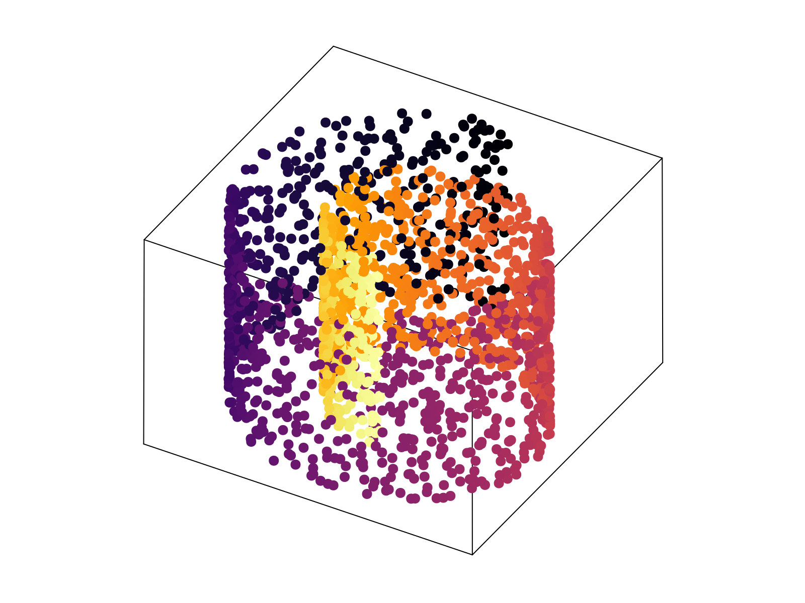
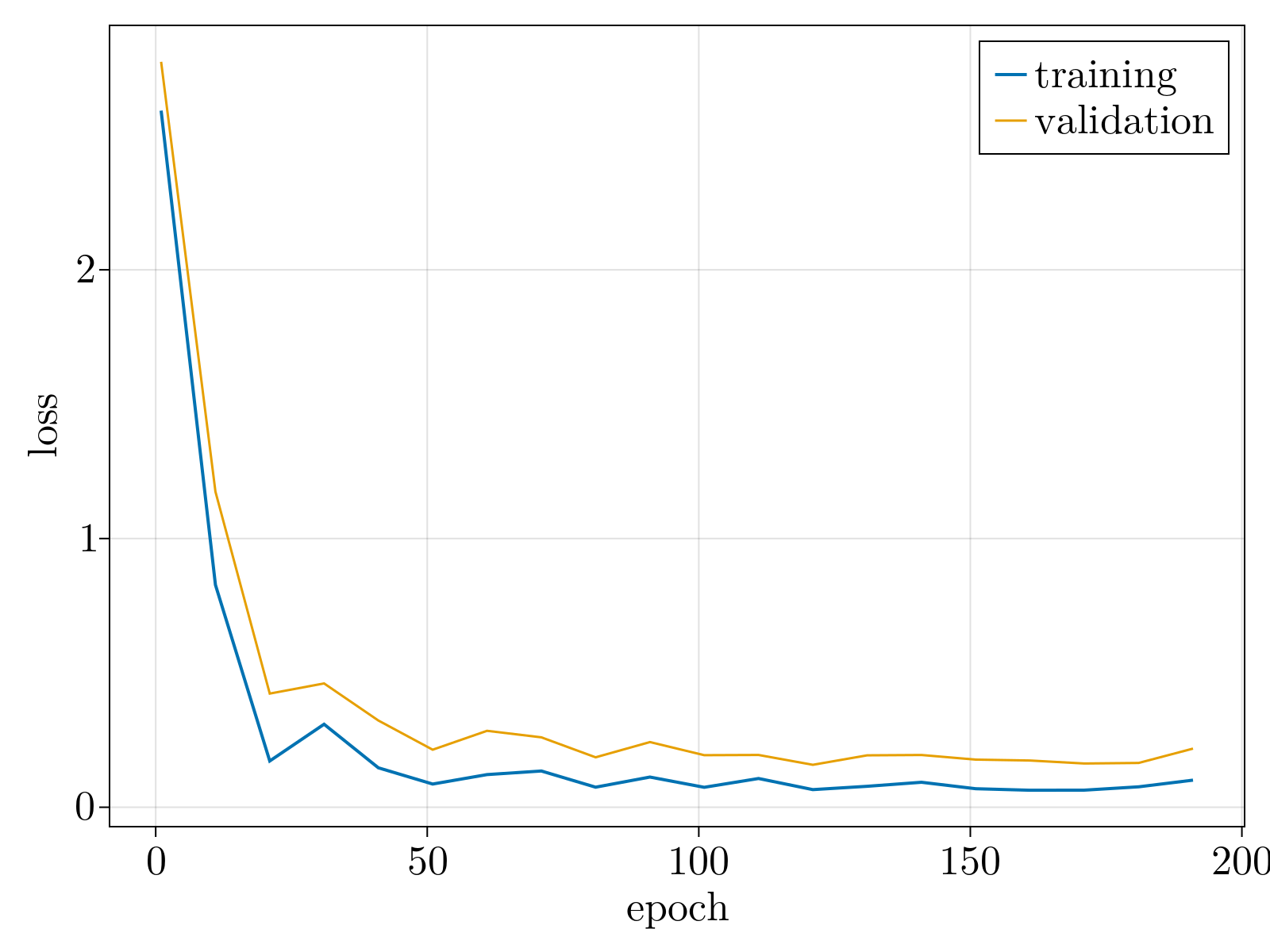
Specifically, we generated a 2D swiss roll, embedded in $30$ dimensions, with $1\%$ random Gaussian noise added to each component. The neural network, as specified in Network objective function, was minimized until convergence (shown above). The resultant 2D latent space, the output of the encoding stage, is shown below after a simple affine transformation to align the $\phi$ axis along the horizontal axis. Importantly, the uniformization constraint results in an approximately linear relationship between the known latent variables used to generate the 2D surface, and the latent parameterization variables.

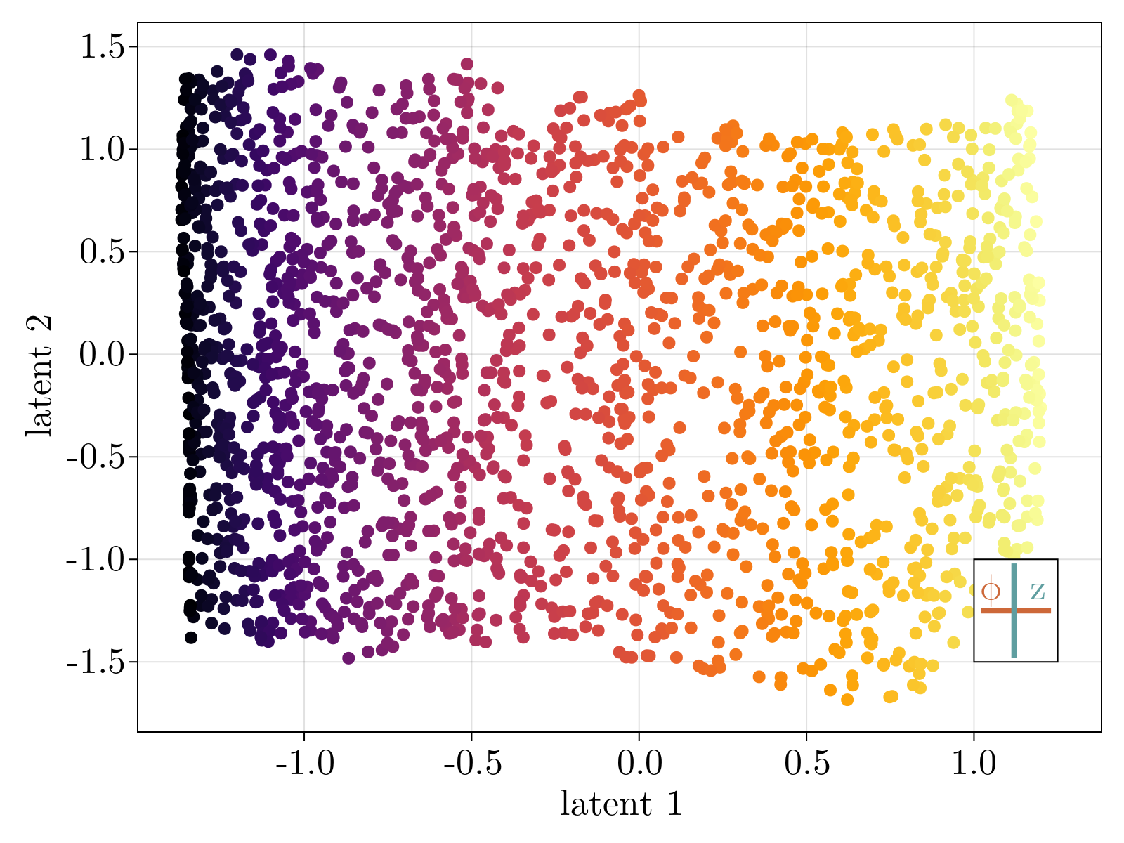
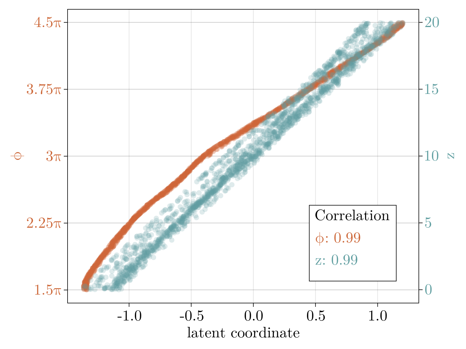
Critically, the output of the decoder stage correlates with the input data such that $R^2 \sim .98$. This held true for 10 independent trained networks with no observed large-scale non-linearity left in the latent space. We conclude that our construction accurately recapitulates the 2D intrinsic parameterization of the toy data.

Drosophila manifold

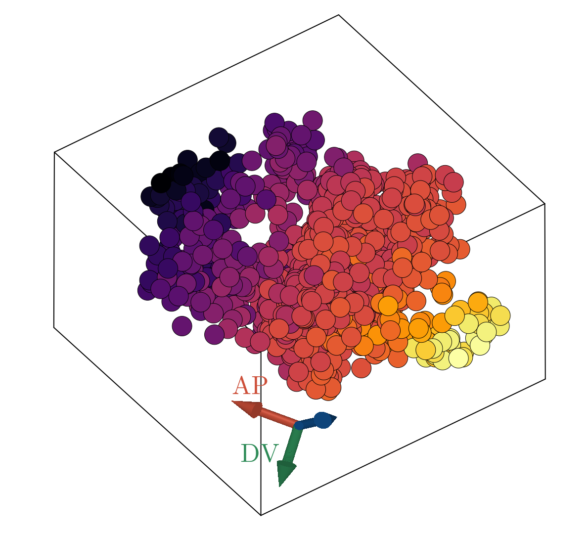
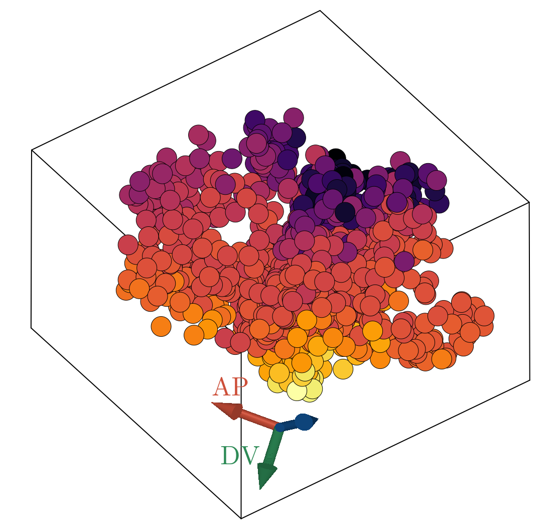
We now show the results of the minimization of the energy specified in Network objective function using the architecture outlined in Network architecture, with three latent dimensions. Below, we show a scatter plot of all scRNAseq cells transformed to the learned latent representation. The left and right plots are colored according to the estimated AP and DV positions respectively, as obtained by scRNAseq spatial inference. We emphasize here that we did not train on the spatial positions, but rather the continuity of space directly follows from imposing the continuity of gene expression in the latent space. Additionally, we did not constrain AP and DV axes, shown as red and green arrows in the triad, to be orthogonal. Rather, we simply looked for the directions in the latent space that maximally correlate with our estimated position. The resultant two directions have negligible overlap. The input data and the output of the decoder stage correlate such that $R^2 \sim .68$, implying we can capture roughly $\sim 70 \%$ of the variance observed in normalized gene expression with just three latent dimensions.

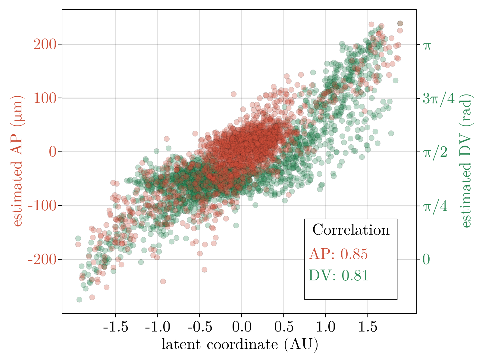
We observe good linear agreement with our estimated AP/DV directions in the latent space and the estimated spatial position for each cell, as shown above. Our ability to resolve AP position is limited to a precision of roughly $.08$mm, much larger than the cellular resolution obtained utilizing FISH data of the 4 gap genes ^[11]. The causal driver behind this is likely multifaceted: (i) scRNAseq is fundamentally noisy (ii) we have a relatively small sized dataset, (iii) our estimates of embryonic position themselves are noisy values. It would be interesting to revisit this analysis leveraging a higher sequencing depth per cell allowable with modern scRNAseq techniques or utilizing novel spatial-omics to provide more exact positional values. Interestingly, our estimated DV axis appears to be qualitatively nonlinear with strongest predictive power at the poles and weak relationship in the bulk.

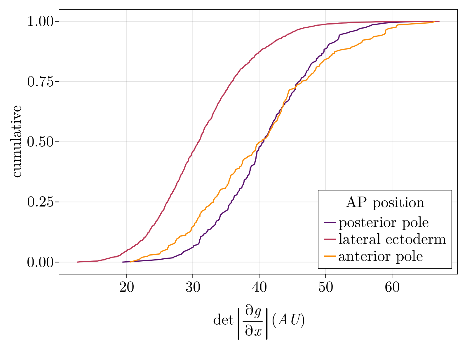
The benefit of using an autoencoder network is that its is both generalizable and generative: we ultimately have a function that maps scRNAseq to a latent space and back out to the original expression domain. For example, we can "generate" novel scRNAseq data from our interpolated model by sampling points in the latent space and transforming the points through the decoder stage. More importantly, this allows us to directly leverage tools from vector calculus to estimate volumes of phase space. As shown in the below right figure, we observe both the anterior and posterior poles contain more "volume" of the gene expression manifold for a unit volume of physical space when compared to cells sampled from the lateral region. Assuming a constant density of states over the intrinsic gene expression manifold, this implies a higher density of cell fates at the head and tail of the embryo than the lateral ectoderm. This is in contrast to previous analyses done on the AP pattern of the 4 gap genes over the mid-sadigittal plane of the embryo which predicted a constant positional information ^[11]. We note that this is an interesting direction for future study.

An interesting question to consider for future studies: what is the third latent dimension we discover within the scRNAseq data? We analyzed the genes that maximally correlate (negatively or positively) with this direction in the latent space, as shown by the blue arrow above. The below table captures some examples of the top hits for both signs. Theses genes are putatively ubiquitously expressed, consistent with the notion that this is an orthogonal axis to the directions of spatial variation. We postulate this direction is involved in the cell cycle as RNApolymerase, myosin light chain, and other mitotic markers form on "pole" of the axis, while ed and other negative growth regulators are enriched on the conjugate pole.